Dataset format

Everything mapcv writes goes into writer.staging_dir. The layout is the same for every source; only the file formats differ (writer.image_format and writer.mask_format). This is a segmentation dataset; detection datasets have boxes instead of masks, instance segmentation datasets a mask per object, classification datasets a label table instead of masks, change detection datasets image pairs and a change mask, and regression datasets float targets.

• Directorydataset/

  • DirectoryImages/

    • patch_0000000.png .png or .jpg (RGB) · .npy · .tif (GeoTIFF)
    • patch_0000001.png
    • patch_0000000.pgw only with world_files: true
    • …
  • DirectoryMasks/ only when the config has labels

    • patch_0000000.png .png (default) · .npy · .tif, same stem as the image
    • …
  • manifest.json
  • patches.geojson footprint of every patch in WGS-84
  • Directorysplits/ only after a split

    • train.txt
    • val.txt
    • test.txt
    • split.json settings and counts of the split
    • Directory10/

      • labeled.txt
      • unlabeled.txt
    • Directory20/

      • …
    • Directory30/

      • …

Files

Naming. Patches are numbered patch_0000000 … in the order they were written (seven digits, zero-padded). The image and its mask share the stem; the extension follows writer.image_format and writer.mask_format, so they can differ: Images/patch_0000042.npy ↔ Masks/patch_0000042.png. Read the paths from each manifest entry’s files rather than building them.

Several imagery sources. With imagery as a list, each source’s patches go to Images/<name>/ under the same stem (Images/before/patch_0000042.tif, Images/after/patch_0000042.tif), every one on the first source’s pixel grid, and the masks stay in Masks/. Each source keeps its own band count and data type. With writer.stack_sources: true the sources share one file per patch instead, Images/patch_0000042.npy of shape (T, C, H, W) (T sources in config order) or a GeoTIFF of T × C bands named <source>_<band>; its files key is image, and the manifest’s writer.stack_sources is true.

	png / jpg	npy	tif
Image	RGB (or gray repeated into three channels), uint8, shape (H, W, 3) when decoded: XYZ tiles, or a uint8 GeoTIFF with 1 or 3 bands	NumPy array in the source’s data type (float32 for EOPF Zarr, uint16 for Sentinel-2 COGs, the file’s for a GeoTIFF), shape (bands, H, W) (bands-first)	GeoTIFF with one band per channel, the source’s data type; reads as (bands, H, W)
Band order	red, green, blue (XYZ) or imagery.bands	exactly imagery.bands	the same, also named in the file (band descriptions)
Values	0–255	as the source stores them: decoded L2A surface reflectance (typically 0–1) for EOPF Zarr, digital numbers for COGs	as the other two
NoData	black (0, 0, 0) pixels (failed tiles, padding, provider NoData)	NaN where an EOPF product has no data, 0 in padded areas; integer data keeps its NoData value	like the source’s format; floating-point GeoTIFFs declare NaN as no-data
Mask	single-channel PNG, uint8 (16-bit PNG for uint16 masks), (H, W)	NumPy array, (H, W), the mask’s own dtype	single-band GeoTIFF, the mask’s own dtype

Masks. 0 is background (imagery, no polygon), other values are class IDs from the manifest’s target.class_map, and 255 (labels.ignore_index, recorded as the manifest’s target.ignore_index) marks pixels with no imagery under them: padding, failed tiles and NoData. Without labels.label_field, every polygon is 1 and class_map is empty. With raster labels, 255 also marks pixels without a label: outside the label raster, its NoData and labels.ignore_values. The values are the same in png, npy and tif. Segmentation and change masks are uint8, instance-ID masks uint16 and regression targets float32 (PNG holds uint8 and uint16). A tif mask also declares ignore_index as its no-data value, so GIS tools and rasterio (read(masked=True)) treat those pixels as missing. Pass the ignore value to your loss; see Use your dataset.

Georeferenced outputs

GeoTIFF patches

With writer.image_format: tif (and writer.mask_format: tif) every patch is a GeoTIFF written by mapcv. Open it in QGIS, with rasterio, GDAL or TerraTorch and it sits in the right place.

Layout	Striped (about 1 MiB of pixels per strip, so a 256 × 256 patch is one strip), pixel-interleaved, little-endian, classic TIFF
Compression	Deflate (zlib) with the horizontal predictor for 8, 16 and 32-bit integers and the floating-point predictor for float32/float64 (64-bit integers: none). 8 and 16-bit data use the fast compressor behind PNG writing (as small as the PNG patches, written about as fast or faster); wider data use zlib level 1, which shrinks float32 bands by about a quarter
Data types	uint8, int8, uint16, int16, uint32, int32, uint64, int64, float32, float64; the data type of the source (images) or the target (masks)
Bands	One per channel. 3-band uint8 and uint16 images are tagged RGB, other counts as grey bands with unspecified extra samples. Band names (red, green, blue, or imagery.bands) are stored as band descriptions
CRS	The source’s crs as an EPSG code (GTModelType, GTRasterType = PixelIsArea, and ProjectedCSType or GeographicType GeoKeys). Only CRSs written EPSG:<code> can be stored
Transform	The patch’s own transform, from the source transform plus the patch’s row and col: identical to Manifest.patch_transform(entry). North-up grids use ModelPixelScale and ModelTiepoint; rotated or south-up grids use ModelTransformation
No-data	Images: the source file’s no-data value for GeoTIFF imagery (imagery.nodata or the file’s own); otherwise NaN for floating-point data and none for integer data (a no-data value applies per band, and 0 is a real value in an RGB band). Masks: labels.ignore_index, when set

An image and the mask of the same patch share one transform bit for bit, so they open aligned. Padded patches at the raster edge keep the transform of their top-left pixel, as in the manifest. patch_shape in the manifest is [bands, H, W] for tif, the shape you get from rasterio’s read().

import rasterio

with rasterio.open("dataset/Images/patch_0000000.tif") as src:
    image = src.read()                  # (bands, H, W), the stored dtype
    print(src.crs, src.transform, src.bounds, src.descriptions)

with rasterio.open("dataset/Masks/patch_0000000.tif") as src:
    mask = src.read(1)                  # (H, W)
    valid = src.read_masks(1) > 0       # False where the value is ignore_index

World files

With writer.world_files: true, every PNG gets a .pgw and every JPG a .jgw file with the same stem, in Images/ and Masks/. A world file has six lines (x pixel size, y rotation, x rotation, y pixel size, then the x and y of the centre of the top-left pixel) and no CRS. GDAL and QGIS find it next to the image and place it; set the CRS from sources[0].crs in the manifest. The files are listed in each entry’s files as image_world (<name>_world for each of several sources) and mask_world. They are not written for npy or tif.

patches.geojson

A GeoJSON FeatureCollection in WGS-84 (longitude, latitude) with one Polygon per patch, in manifest order, written after the split so each feature knows its split. The ring is the patch’s four corners, converted from the source CRS, counter-clockwise and closed.

dataset/patches.geojson (one feature)

{"type":"Feature","properties":{"filename":"patch_0000000.png","split":"train","row":0,"col":0,"padded":false,"empty_ratio":0.0,"class_pixels":{"0":54098,"1":11438}},"geometry":{"type":"Polygon","coordinates":[[[4.98230,52.41127],[4.98428,52.41127],[4.98428,52.41228],[4.98230,52.41228],[4.98230,52.41127]]]}}

Property	Meaning
filename	The name the split lists use (the file name of the image)
split	train, val or test; null without a split, or for a patch a spatial split dropped
row, col, padded, empty_ratio	As in the manifest entry
class_pixels	Mask pixels per class ID, as in the manifest summary (segmentation and change)

mapcv split rewrites the file’s split properties when it finds one. Turn the file off with writer.footprints: false (a million patches make a file of several hundred MB). Coordinates have nine decimals (about 0.1 mm). CRSs other than Web Mercator and WGS-84 are converted with pyproj.

manifest.json

A JSON object describing the dataset once (task, imagery source, target, writer, sampler) and then every patch. mapcv 0.3 writes version 3. Manifest.load, mapcv info and mapcv split also read version 2 (mapcv 0.2) and version 1 (mapcv 0.1) and upgrade them in memory; see Older versions.

The dataset-wide blocks are indented; each patch is one line, so a manifest with 100,000 patches stays about 20 MB and diffs line by line.

dataset/manifest.json (first two patches)

{
  "version": 3,
  "mapcv_version": "0.3.0",
  "complete": true,
  "task": "segmentation",
  "sources": [
    {
      "name": "image",
      "source_type": "xyz",
      "product_id": "esri_satellite",
      "bands": ["red", "green", "blue"],
      "dtype": "uint8",
      "crs": "EPSG:3857",
      "transform": [0.5971642834779232, 0.0, 549582.2333704159,
                    0.0, -0.5971642834774684, 6868784.235762509],
      "patch_shape": [256, 256, 3],
      "width": 2048,
      "height": 1536
    }
  ],
  "target": {
    "type": "segmentation",
    "class_map": { "building": 1 },
    "ignore_index": 255,
    "dtype": "uint8",
    "labels": {
      "label_field": "class", "classes": null, "all_touched": false,
      "sha256": "a1bfc9b00f10d47298fca03c087a1373f6d5af02810a514cd97b3a056d0bded4"
    },
    "options": {}
  },
  "writer": { "layout": "files", "image_format": "png", "jpg_quality": 95, "jpg_subsampling": "4:2:0", "mask_format": "png" },
  "sampler": {
    "patch_size": 256, "stride": 256, "mode": "grid", "edge_strategy": "drop",
    "pad_mode": "zero", "max_empty_ratio": 1.0, "min_label_ratio": 0.0,
    "random_seed": 42, "random_count": 100
  },
  "patches": [
    {"row":0,"col":0,"padded":false,"chunk":0,"files":{"image":"Images/patch_0000000.png","mask":"Masks/patch_0000000.png"},"summary":{"class_pixels":{"0":54098,"1":11438},"empty_ratio":0.0}},
    {"row":0,"col":256,"padded":false,"chunk":0,"files":{"image":"Images/patch_0000001.png","mask":"Masks/patch_0000001.png"},"summary":{"class_pixels":{"0":43080,"1":22456},"empty_ratio":0.0}}
  ]
}

Top-level fields

Field	Type	Meaning
version	int	3. A reader refuses a higher version with a message to upgrade mapcv
mapcv_version	string | null	The mapcv that created the dataset (a resumed run keeps it). null for a manifest upgraded from version 1 or 2
complete	bool	false while mapcv generate writes the dataset and after it stopped early (Ctrl-C, a failed chunk, a full disk); true once every patch, the splits and the annotation files are written. mapcv info and mapcv verify report an incomplete dataset; running mapcv generate again with the same config finishes it. Absent in manifests written before mapcv 0.3, which did not record it
task	string	The config’s task: "segmentation", "detection", "instance", "classification", "change" or "regression"
sources	list	The imagery, one object per source: one named "image", or the configured sources in order. See Sources
target	object | null	What each patch is annotated with. null for an image-only dataset (no labels). See Target
writer	object	How patches are stored: layout ("files": one file per patch in Images/ and Masks/; "change" for change datasets), image_format (png, jpg, npy or tif), jpg_quality, jpg_subsampling and mask_format (png, npy or tif; absent for detection, classification and instance datasets without instance.id_mask), plus world_files: true and stack_sources: true when they are on. A resume notices a format change
sampler	object	The resolved sampler config (with stride filled in). Used for resume checks, spatial splits and patch bounds
region	object	Only with an area of interest (region.path): aoi_sha256, the SHA-256 of the polygon file, plus name_field and layer when they are set. A resume refuses edited polygons
patches	list	One entry per patch, in file order. See Patch entries

Sources

Field	Type	Meaning
name	string	The source’s name, and the key of its patch in each entry’s files: "image" for one imagery block, else the configured name
source_type	string	"xyz", "eopf_zarr", "stac_cog" or "geotiff" (Earth Engine imagery is "xyz")
product_id	string | null	XYZ: the built-in source name, custom-xyz:<hostname> for a url_template (the template itself is never stored), or earth-engine:<asset> for Earth Engine. EOPF Zarr: the product’s file name. stac_cog: the STAC item ID. GeoTIFF: the file name (from a URL, its last path segment); for a mosaic, the glob pattern and the number of files (tiles/*.tif (12 files))
bands	list of strings	Channel names in storage order: red, green, blue (XYZ), the configured Sentinel-2 bands or asset keys, or b1, b2, … for a GeoTIFF (the file’s 1-based band numbers)
dtype	string	The stored data type: "uint8" (XYZ), "float32" (EOPF Zarr), the COGs’ type (stac_cog, "uint16" on Earth Search) or the file’s (GeoTIFF)
crs	string	Raster CRS: EPSG:3857 for XYZ, the product’s UTM zone (for example EPSG:32631) for Sentinel-2, the file’s CRS for a GeoTIFF
transform	6 floats	Affine (a, b, c, d, e, f) of the whole raster: x = a·col + b·row + c, y = d·col + e·row + f, in crs units (metres) at the pixel’s top-left corner
patch_shape	list of int	Shape of one stored image patch: [H, W, 3] for PNG/JPG, [bands, H, W] for NPY and TIF
width, height	int	Size in pixels of the raster the patches are cut from: the source’s window over the region. A resume refuses another region on the same grid. Absent in manifests written before mapcv 0.3
factor, offset	int, [row, col]	Only for a further source whose own grid differs from the first source’s: each of its pixels is factor × factor first-source pixels (repeated onto the grid), and its pixel (0, 0) starts at first-source pixel offset. transform stays the source’s own. Every patch, whichever source, is georeferenced by the first source’s transform
fingerprint	object	Identifies the input so a resumed run refuses a different one; absent for built-in XYZ sources and for an EOPF product named by path without scl_mask. Custom XYZ (url_template): url_template_pbkdf2, a salted PBKDF2-SHA256 hash (100,000 rounds) of the template, so another layer, year or style on the same host is refused while a key in the template cannot be read back. GeoTIFF: kind: "file" with size, mtime_ns (the modification time in nanoseconds: pixels edited in place keep the size and both ends of the file) and sha256_head_tail, the SHA-256 of its first and last 64 KiB (the path is not recorded, so a moved file still resumes, as does a copy that keeps its times, such as cp -p or rsync -a), or kind: "url" with the url, the etag and total size the server reports, and sha256_head of the first 64 KiB; both add overview, bands (1-based) and the effective nodata. Nothing reads the whole file. Mosaic: kind: "mosaic" and files, each file’s name and fingerprint, plus overview, bands and nodata. STAC (stac_cog, or eopf_zarr with search): stac with the catalog, collection and item. Sentinel-2 with scl_mask: scl_mask, the masked classes. Earth Engine: earth_engine, the image and rendering settings without project

Target

Field	Type	Meaning
type	string	The kind of annotation: "segmentation" (a class mask per patch), "detection" (boxes), "instance" (a mask per object), "classification" (labels per patch), "change" (a change mask per pair) or "regression" (float targets)
class_map	object	Label value → class ID (mask value, COCO category_id). Empty when every polygon is class 1
ignore_index	int | null	Mask value of pixels without imagery (labels.ignore_index) and, with raster labels, without a label (outside the label raster, its NoData and ignore_values); null when they are background, and for detection and instance. Classification keeps the setting (it decides which pixels are valid)
dtype	string | null	Data type of the mask values: "uint8" for segmentation and change; "float32" for regression; "uint16" for instance datasets with instance.id_mask; null for detection, classification and for instance datasets without ID masks
labels	object	The labels settings (without the path and the mask settings) plus the sha256 of the label file (for a Shapefile also covering its .dbf, .prj and .cpg), so a resume notices edited labels. layer appears when a GeoPackage layer was chosen. For raster labels ("type": "raster") the settings are band, classes (each value as {"id", "name"}), nodata, ignore_values, unmapped and resampling, plus a fingerprint that identifies the label raster as a GeoTIFF source’s does (size and sha256_head_tail for a local file; url, etag, size and sha256_head for a URL) instead of a sha256, since nothing reads the whole file
options	object	Task-specific settings: empty for segmentation and regression; the resolved detection block for detection, the resolved instance block for instance, the resolved classification block for classification, {"change_value": …} for change

Patch entries

Field	Type	Meaning
row, col	int	Top-left pixel of the patch in the whole raster. Can point past the edge for edge_strategy: pad
padded	bool	Part of the patch lies outside the raster and was filled by pad_mode
chunk	int	Index of the processing chunk that wrote the patch (used to resume)
files	object	Role → path of the patch’s files, relative to the dataset folder with / separators: each source’s name (image for one imagery block) and, with labels, mask (instance datasets: only with instance.id_mask); with world_files, image_world (<name>_world per source) and mask_world
summary	object	What the patch holds, readable without opening it: empty_ratio (fraction of empty pixels, black RGB or NaN in any band, 0–1) and, with labels, class_pixels (mask pixel count per class ID as strings, ascending, the ignore value included: {"0": 54098, "1": 11438, "255": 512}). Detection and instance datasets have class_objects instead: the number of boxes or masks per class ID, as strings, ascending ({"1": 12, "3": 2}; {} for a patch without objects). Classification datasets have class_coverage, each class’s share of the patch’s valid pixels (class IDs as strings, ascending; classes without pixels are left out: {"1": 0.375, "3": 0.0625}), and labels, the class IDs the patch was given, ascending ([1]; [0] is the background label). Regression datasets have values (see Regression datasets). With an area of interest, every entry also has region, the name of the region that covers most of the patch

Readers should ignore keys they do not know: later 0.3 releases may add keys (new tasks add files roles and summary keys) without changing version. Renaming or removing a key changes version.

Georeferencing

Patch transforms and footprints are not stored per patch; they follow exactly from row, col and the source’s transform, so storing them would only make the manifest bigger. mapcv.Manifest.patch_transform(entry) and patch_bounds(entry) compute them, or by hand. GeoTIFF patches, world files and patches.geojson are all derived from the same transform, so they agree with these:

import json

manifest = json.loads(open("dataset/manifest.json").read())
source = manifest["sources"][0]
a, b, c, d, e, f = source["transform"]
size = manifest["sampler"]["patch_size"]
patch = manifest["patches"][0]
left, top = c + a * patch["col"], f + e * patch["row"]
right, bottom = left + a * size, top + e * size
print(source["crs"], (left, bottom, right, top))

Older versions

Manifest.load upgrades older manifests in memory and never rewrites the file; Manifest.load(path).save(path) converts one to version 3 on disk.

Version	Written by	Upgraded as
2	mapcv 0.2	filename/mask_filename become files (Images/…, Masks/…), strip_index becomes chunk, per_class_pixel_counts and empty_ratio move into summary, the source fields into sources[0], class_map and labels into target. mapcv 0.2 had no ignore index, so target.ignore_index is null (a labels.ignore_index recorded by a 0.3 development build is kept). writer gains layout: files, mask_format: png and jpg_subsampling ("4:4:4" for JPEG patches, which 0.2 wrote with full-resolution colour; "4:2:0" otherwise). mapcv_version is null
1	mapcv 0.1	As version 2, without sampler, writer, labels, crs and transform; row is relative to a strip, not the raster

A version-2 dataset can be split, inspected and resumed by mapcv 0.3 when its settings match the config, with labels.ignore_index: null because 0.2 wrote background where there is no imagery. A finished 0.2 dataset is left untouched; a resumed one that gains patches is saved as version 3. Version-1 datasets, and version-2 datasets made with sampler.mode: random (0.3 draws random anchors differently), can be split and inspected but not resumed. Details: Migrating to 0.3.

Detection datasets

With task: detection the images go to images/ and each patch’s objects become boxes in COCO JSON and YOLO text files (the detection.formats you chose). There are no masks.

• Directorydataset/

  • Directoryimages/

    • patch_0000000.png same naming and encoding as above
    • …
  • Directorylabels/ YOLO

    • patch_0000000.txt one line per object; no file for a patch without objects
    • …
  • Directoryannotations/ COCO

    • instances_train.json
    • instances_val.json
    • instances_test.json instances_all.json instead when there is no split
    • Directoryobjects/ the exact boxes per processing chunk, which the files above are built from

      • …
  • train.txt YOLO image lists: ./images/patch_….png
  • val.txt
  • test.txt
  • dataset.yaml Ultralytics dataset file (written with a split)
  • patches.geojson footprints, as for segmentation (writer.footprints)
  • manifest.json
  • Directorysplits/

    • …

Detection uses the same writer settings as segmentation, except mask_format, which is an error to set (there are no masks). image_format: tif writes GeoTIFF images (Ultralytics reads them; COCO’s file_name ends in .tif), world_files adds a world file next to PNG/JPG images (files.image_world), and patches.geojson is written and kept in step with mapcv split as for any dataset.

What an object is. One label feature is one object: a MultiPolygon is one object, and a feature cut into pieces by a patch edge is one object whose box covers every visible piece. Its box is the axis-aligned bounding box of the part that is visible in the patch: inside the patch, inside the raster (not in padding) and over pixels with imagery (failed tiles and NoData are cut out). Holes do not change a box. An object is kept when at least min_visible of its area is visible and the box is at least min_box_pixels wide and high; point features become point_box_size squares when that is set.

Coordinates. Boxes are in pixels of the patch, with the origin at its top-left corner: x to the right, y down, continuous, so pixel (col, row) covers [col, col+1] × [row, row+1] and a box spans at most [0, patch_size]. Values are rounded to 1/10,000 of a pixel.

COCO

One file per split, each a standard COCO detection document (pycocotools.coco.COCO(path) loads it; so do torchvision’s CocoDetection, Detectron2 and MMDetection). The image root is images/.

dataset/annotations/instances_train.json (shortened)

{
  "info": {"description": "mapcv object detection dataset, train patches", "mapcv_version": "0.3.0"},
  "licenses": [],
  "categories": [
    {"id": 1, "name": "building", "supercategory": "object"}
  ],
  "images": [
    {"id": 1, "file_name": "patch_0000000.png", "width": 256, "height": 256}
  ],
  "annotations": [
    {"id": 1, "image_id": 1, "category_id": 1, "bbox": [12.4021, 0.0, 30.1157, 17.9002], "area": 431.0863, "iscrowd": 0, "truncated": true}
  ]
}

Field	Meaning
images[].id	The patch number + 1 (patch_0000041.png is image 42), the same in every split file and after mapcv split
images[].file_name	The image’s file name in images/
annotations[].id	Objects numbered from 1 over all patches in manifest order, so an object keeps its ID whichever split it lands in
category_id	The class ID from target.class_map; 1 (named object) without labels.label_field
bbox	[x, y, width, height] in patch pixels (see above)
area	The visible area of the object in square pixels (not the box area), as COCO’s evaluation expects
iscrowd	Always 0
truncated	true when part of the object is not visible in this patch: cut by the patch or raster edge, or over pixels without imagery. Not part of the COCO standard; tools ignore it

Images without objects are listed with no annotations, so evaluation counts their false positives. categories lists every class of the class map, ascending by ID, even one without objects.

YOLO

labels/<image stem>.txt has one line per object, class cx cy w h: the class index, the box centre and the box size, each divided by the patch size, so between 0 and 1. Class indices are 0-based in ascending class-ID order: with {building: 1, road: 2}, building is 0 and road is 1. A patch without objects has no label file, Ultralytics’ convention for background images.

dataset/labels/patch_0000000.txt

0 0.1072654297 0.0349613281 0.1176394531 0.0699226563

dataset.yaml follows Ultralytics’ format: train, val and test are the image lists next to it, and names maps class indices to names. It has no path key, so Ultralytics takes the dataset root from the folder that holds dataset.yaml: the dataset can be moved or copied to another machine as a whole folder and still trains. (A relative path would be resolved against the working directory or Ultralytics’ own datasets folder, and an absolute one breaks on another machine.) Ultralytics finds each image’s labels by replacing /images/ with /labels/ in its path, which is why detection images live in images/.

dataset/dataset.yaml

train: train.txt
val: val.txt
test: test.txt
names:
  0: building

dataset.yaml and the image lists need a split; without one mapcv writes instances_all.json and the YOLO label files and warns. mapcv split rebuilds the COCO files, the lists and dataset.yaml for the new split, with the same IDs.

annotations/objects/

One JSON file per processing chunk (chunk_000012.json, the manifest entries’ chunk): {"chunk": 12, "patches": {…}}, where patches maps each patch’s image file name to its objects as [category_id, x, y, width, height, area, truncated]. They are written next to the images, so an interrupted run resumes and mapcv split re-splits without recomputing any box. Read the COCO or YOLO files instead; this folder is mapcv’s own.

Instance segmentation datasets

With task: instance the images go to images/ and each patch’s objects become one binary mask each, stored as run-length encoded (RLE) segmentations in COCO JSON. There are no class masks and no YOLO files; with instance.id_mask each patch also gets a 16-bit instance-ID PNG in masks/.

• Directorydataset/

  • Directoryimages/

    • patch_0000000.png same naming and encoding as above
    • …
  • Directorymasks/ only with instance.id_mask: true

    • patch_0000000.png 16-bit: 0 = background, k = the k-th annotation of the image (writer.mask_format may also be npy or tif)
    • …
  • Directoryannotations/ COCO

    • instances_train.json
    • instances_val.json
    • instances_test.json instances_all.json instead when there is no split
    • Directoryobjects/ the instances per processing chunk, which the files above are built from

      • …
  • patches.geojson footprints, as for segmentation (writer.footprints)
  • manifest.json
  • Directorysplits/

    • …

Instance datasets use the same writer settings as segmentation, except that mask_format is an error to set without id_mask. world_files adds a world file next to PNG/JPG images and, with id_mask, next to PNG masks.

What an instance is. One label feature is one instance: a MultiPolygon is one instance, and a feature cut into pieces by a patch edge is one instance whose mask covers every visible piece. Its mask holds the pixels of the feature that are inside the patch, inside the raster (not in padding) and over pixels with imagery (failed tiles and NoData are cut out). Holes are holes. An instance is kept when at least min_visible of its area is visible and its mask has at least min_area pixels.

Exact masks. Each instance is rasterized on its own, on the patch’s pixel grid, with the rasterizer that writes segmentation masks (a port of GDAL’s: a pixel is burned when its centre is inside the polygon, with labels.all_touched when an edge passes through it). The instances of a patch may overlap, and every mask is exact: nothing overwrites anything. With min_visible: 0 and min_area: 1 (every instance kept), painting them in feature order gives the segmentation mask of the same labels over the pixels that have imagery.

COCO

One file per split, each a standard COCO instance segmentation document (pycocotools.coco.COCO(path) loads it, and coco.annToMask(ann) decodes an annotation; so do torchvision’s CocoDetection, Detectron2 and MMDetection). The image root is images/.

dataset/annotations/instances_train.json (shortened)

{
  "info": {"description": "mapcv instance segmentation dataset, train patches", "mapcv_version": "0.3.0"},
  "licenses": [],
  "categories": [
    {"id": 1, "name": "building", "supercategory": "object"}
  ],
  "images": [
    {"id": 18, "file_name": "patch_0000017.png", "width": 256, "height": 256}
  ],
  "annotations": [
    {"id": 33, "image_id": 18, "category_id": 1, "segmentation": {"size": [256, 256], "counts": "baV13m78H00000^Vh0"}, "bbox": [154, 50, 5, 11], "area": 47, "iscrowd": 0, "truncated": false}
  ]
}

Field	Meaning
images[].id, file_name	As for detection: the patch number + 1, stable in every split file and after mapcv split; the image’s file name in images/
annotations[].id	Instances numbered from 1 over all patches in manifest order (feature order within a patch), so an instance keeps its ID whichever split it lands in
category_id	The class ID from target.class_map; 1 (named object) without labels.label_field
segmentation	The mask as a compressed RLE: size is [height, width] of the patch and counts the run lengths as the string pycocotools.mask.encode writes. Runs go down each column in turn (column-major order), alternate between background and the instance, and start with background (a zero-length run when the first pixel is in the instance). The mask equals the one the instance’s bbox and area describe
bbox	[x, y, width, height], the tight box around the mask’s pixels, as integers in patch pixels (the same as pycocotools.mask.toBbox)
area	The number of pixels in the mask (the same as pycocotools.mask.area)
iscrowd	Always 0: every instance is one object, stored as RLE
truncated	true when part of the feature is not visible in this patch: cut by the patch or raster edge, or over pixels without imagery. Not part of the COCO standard; tools ignore it

Images without instances are listed with no annotations. categories lists every class of the class map, ascending by ID.

Instance-ID masks

With instance.id_mask: true, masks/<image stem>.png is a 16-bit grayscale PNG (or an .npy or GeoTIFF of uint16, per writer.mask_format) the size of the patch: 0 is background and k marks the pixels of the k-th annotation of that image, numbered from 1 in the order of the annotations (ascending id, which is feature order). Where instances overlap, the later one wins, as later polygons overwrite earlier ones in segmentation masks; an instance that is fully covered by later ones has no pixel in the PNG but keeps its exact COCO mask. A patch with more than 65,535 instances stops the run with an error that names the fixes (a smaller patch size, a larger min_area, or no ID masks). The manifest lists the file as files.mask.

annotations/objects/

As for detection, one JSON file per processing chunk maps each patch’s image file name to its instances, as [category_id, x, y, width, height, area, truncated, counts]. They are written next to the images, so an interrupted run resumes and mapcv split re-splits without rasterizing again. Read the COCO files instead; this folder is mapcv’s own.

Classification datasets

With task: classification the images go to images/ and the labels to flat tables next to them, as EuroSAT and BigEarthNet are laid out. There are no masks. How a label is decided: classification.

• Directorydataset/

  • Directoryimages/

    • patch_0000000.png same naming and encoding as above
    • …
  • labels.csv image,labels, plus split once the dataset has a split
  • labels_train.csv image,labels of one split; only with a split
  • labels_val.csv
  • labels_test.csv
  • classes.txt one class name per line, in class ID order
  • labels.json {"classes": [...], "images": {"patch_0000000.png": ["building"]}}
  • patches.geojson footprints, as for segmentation (writer.footprints)
  • manifest.json
  • Directorysplits/

    • …

Classification uses the same writer settings as segmentation, except mask_format, which is an error to set. image_format: tif writes GeoTIFF images, world_files adds a world file next to PNG/JPG images and patches.geojson is written and kept in step with mapcv split as for any dataset.

dataset/labels.csv

image,labels,split
patch_0000000.png,farmland,train
patch_0000001.png,built_up farmland,train
patch_0000002.png,background,val
patch_0000003.png,forest,

• image is the file name inside images/ (the name the split lists use). Rows follow the manifest’s patch order, which is the order of the patch numbers.
• labels holds the patch’s class names, joined by one space for mode: multi (a single name for single; CSV quoting applies where a name has a comma, a quote or, with single, a space). It is never empty: a patch without a label is not written (empty: skip) or is background. Split it on spaces for a multi-label dataset.
• split is train, val or test, and empty for a patch a spatial split left out. It appears once the dataset has a split, and mapcv split rewrites it.
• labels_<split>.csv hold the same image,labels rows of the patches of one split (manifest order); they exist only while the dataset has a split.
• classes.txt lists the class names in ascending class ID order, one per line, with background first when classification.empty is background. A name’s line number is not its ID when the IDs have gaps; the manifest’s target.class_map gives the IDs.
• labels.json has the same names as classes and, for every image, its labels as an array (also for single-label datasets). It does not depend on the split.

All files are UTF-8 with \n line ends on every OS, and the same config gives the same bytes. The tables are built from the manifest (class_coverage and labels of each entry’s summary), so a resumed run or mapcv split rewrites them for every patch. To build a multi-hot vector, use the order of classes.txt:

import json

import numpy as np

data = json.load(open("dataset/labels.json"))
index = {name: i for i, name in enumerate(data["classes"])}
target = {image: np.isin(np.arange(len(index)), [index[name] for name in names]).astype("float32")
          for image, names in data["images"].items()}

Change detection datasets

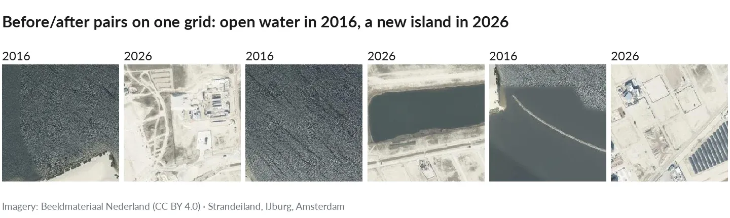
Before/after pairs as a change dataset holds them: the same patch from two imagery sources on one grid, here PDOK’s 2016 and 2026 aerial photos of Strandeiland, an island raised from the water in between (Beeldmateriaal Nederland, CC BY 4.0).

With task: change each patch is a pair of images, before and after, with a change mask, in the folder layout of LEVIR-CD that change-detection loaders read:

dataset/
├── A/            the before image (the first imagery source): patch_0000000.png …
├── B/            the after image (the second source), same file names
├── label/        the change mask, same file names
├── splits/       train.txt, val.txt, test.txt: the file names in each split
├── patches.geojson
└── manifest.json

The three files of a patch share their name and grid: A/patch_0000042.png, B/patch_0000042.png and label/patch_0000042.png. Each image keeps its source’s band count and data type (writer.image_format applies to both). A mask holds 0 (no change), change.change_value (1 by default) for changed pixels and the ignore value (255 by default) where either image has no imagery or a change raster has no label; writer.mask_format sets its format as for segmentation. Splits stay lists of names, so mapcv split rewrites splits/ without moving any file; a loader that wants train/A/… folders can follow the lists.

In the manifest, task is change, writer.layout is change, sources holds the two images (files keys are their names, plus mask) and target.class_map is {"change": <change_value>}. target.labels holds the settings and hash of the change labels or, for two label sets, {"before": …, "after": …}; target.options.change_value the change value. Each entry’s summary.class_pixels counts the mask’s values, as for segmentation, and stratified splits use it.

Regression datasets

With task: regression the layout is the segmentation one, Images/ and Masks/, but each “mask” is a float32 target: a single-band GeoTIFF (writer.mask_format: tif, the default for regression, which declares NaN as its no-data value) or an (H, W) NPY array. A pixel holds value × labels.scale + labels.offset of the continuous raster at its centre, and NaN where there is no value (outside the raster, NoData, out-of-range values, no imagery). Mask the NaN pixels out of your loss, for example loss = mse(pred[valid], target[valid]) with valid = ~torch.isnan(target).

In the manifest, task is regression, target.dtype is float32, target.class_map is empty and target.ignore_index is null (NaN plays its part). target.labels holds the raster settings, scaling included, and the raster’s fingerprint. Each entry’s summary.values is {valid, min, max, mean}: the number of pixels with a value and, when there are any, their statistics (computed in float64). Several imagery sources and writer.stack_sources work as for segmentation.

Split files

File	Content
splits/train.txt, val.txt, test.txt	Patch names, one per line: the file name of each entry’s first source (files.image for one source, patch_0000123.png)
splits/<percent>/labeled.txt	The first ⌈ratio × len(train)⌉ names of a shuffled train.txt
splits/<percent>/unlabeled.txt	The rest of train.txt
splits/split.json	The split settings (SplitterConfig), the strategy actually used, and the train/val/test/dropped counts

<percent> is the labeled ratio as a percentage: 0.1 → 10/, 0.125 → 12.5/. The three main lists are disjoint. With the spatial strategy, some patches may be in no list: they overlapped a held-out patch and were left out of train/val (the count is reported as “overlapping patches left out”). With sample_limit, patches outside the sample are in no list either.

Each list has one name per line and ends with a newline, so wc -l counts patches.

dataset/splits/split.json

{
  "settings": {
    "test_ratio": 0.2,
    "val_ratio": 0.1,
    "labeled_ratios": [0.1, 0.2, 0.3],
    "seed": 42,
    "strategy": "spatial",
    "block_size": null,
    "sample_limit": null
  },
  "strategy_used": "spatial",
  "train": 52,
  "val": 8,
  "test": 17,
  "dropped": 0
}

strategy_used differs from settings.strategy only when a spatial split of a mapcv 0.1 manifest fell back to stratified.

Files added on request

generate writes none of these; the commands below add them to the dataset folder.

File	Written by	Content
stats.json	mapcv stats	Per-band statistics of each source and the class balance, over one split
README.md	mapcv card	A dataset card with Hugging Face YAML metadata
terratorch.yaml	mapcv export --format terratorch	The data: section of a TerraTorch training config (unless --out names another file)
SHA256SUMS	mapcv verify --write-checksums	<sha256> <path> per line (the sha256sum format) for every file in the dataset folder

dataset/stats.json (abridged)

{
  "mapcv_version": "0.3.0",
  "task": "segmentation",
  "split": "train",
  "patches": 36,
  "sources": {
    "image": {
      "bands": ["b1", "b2", "b3"],
      "mean": [124.99, 124.60, 125.00],
      "std": [71.82, 71.85, 71.78],
      "min": [1.0, 1.0, 1.0],
      "max": [249.0, 249.0, 249.0],
      "pixels": [147456, 147456, 147456]
    }
  },
  "classes": {
    "pixels": {"background": 124479, "a": 22977},
    "frequency": {"background": 0.844, "a": 0.156},
    "median_frequency_weights": {"background": 0.769, "a": 1.43}
  }
}

• split is the split counted (all when the dataset has no split lists). pixels counts the pixels each band’s values were taken over; a band without any is null in mean, std, min and max.
• With writer.stack_sources, each source of the stack still has its own entry.
• classes holds pixels, frequency and median_frequency_weights for segmentation and change, objects for detection and instance, and patches for classification; class names come from target.class_map, with background for 0.
• A regression dataset has targets instead: mean, std, min, max and pixels of the target values.