Instance segmentation datasets

This tutorial builds an instance segmentation dataset from the quickstart data: Esri World Imagery over Amsterdam’s Eastern Docklands at about 0.36 m per pixel, with every OpenStreetMap building as its own mask. A semantic mask says which pixels are “building”; an instance mask says which pixels belong to this building, so touching and overlapping buildings stay separate objects. mapcv writes the masks as COCO JSON with RLE segmentations, so the same folder trains with torchvision, Detectron2 or MMDetection.

Time: about 15 minutes. You need: pip install mapcv; pycocotools to read the masks; torch + torchvision for the training step.

1. Get the labels

   The labels are the quickstart’s building outlines (967 features, each with class: building):

   mkdir docklands-masks && cd docklands-masks
   curl -LO https://raw.githubusercontent.com/tahamukhtar20/mapcv/main/examples/quickstart/buildings.geojson

   OSM data is © OpenStreetMap contributors under the ODbL, which asks you to credit it when you share the result.

2. Write the config

   It is the quickstart config plus task: instance and an optional instance block. mapcv init --template instance writes the same file with comments.

   mapcv.yaml

   task: instance
   
   region:
     west: 4.9375
     south: 52.3725
     east: 4.9515
     north: 52.3780
   
   imagery:
     type: xyz
     zoom: 18                   # ≈ 0.36 m/px at this latitude
     source: esri_satellite
     max_connections: 4
   
   labels:
     path: buildings.geojson
     label_field: class         # one class: building
   
   instance:
     min_visible: 0.3           # keep a building in a patch if ≥ 30% of it is visible there
     min_area: 4                # drop masks with fewer than 4 pixels
     id_mask: true              # also write one 16-bit instance-ID PNG per patch
   
   sampler:
     patch_size: 256
     edge_strategy: drop
   
   writer:
     staging_dir: ./dataset
     image_format: png
   
   split:
     strategy: spatial          # whole blocks per split: no leakage between splits
     test_ratio: 0.20
     val_ratio: 0.10
     seed: 42

   How a building becomes a mask:

   • One feature, one instance. Each label feature (GeoJSON, KML, GeoPackage, Shapefile or GeoParquet) is one instance, including a MultiPolygon. A building cut by a patch edge is still one instance; its mask is the part inside the patch.
   • Exact masks. Every building is burned on its own, with the rasterizer and the pixel rule that write segmentation masks: a pixel belongs to a building when its centre is inside the footprint (labels.all_touched: true also takes every pixel an edge passes through). Because buildings are not burned into one shared mask, two overlapping footprints each keep their exact mask. Courtyards (holes) stay empty.
   • Only what is visible. The mask holds the pixels of the building that are inside the patch, inside the raster, and over pixels that have imagery (failed tiles and NoData are cut out).
   • min_visible decides whether a building that the patch shows only in part gets a mask there. With 0.3, a building split 50/50 between two patches gets a mask in both, and one with 20% in a patch gets none in that patch. Masks of cut buildings are flagged truncated in COCO.
   • min_area removes slivers along patch edges and buildings smaller than a few pixels.
   • id_mask adds the instance-ID PNG described below. Leave it off if COCO is all you need.

   All options: Configuration → instance.

3. Plan

   $ mapcv plan mapcv.yaml
   ╭─ Plan for mapcv.yaml ────────────────────────────────────────────────────────╮
   │ Task     instance · COCO RLE masks · min_visible 0.3 · masks ≥ 4 px ·        │
   │          instance-ID PNGs                                                    │
   │ Region   4.9375, 52.3725 → 4.9515, 52.378  (≈ 1.0 × 0.6 km)                  │
   │ Imagery  esri_satellite · zoom 18 (≈ 0.36 m/px)                              │
   │ Raster   2,816 × 1,792 px · 77 tiles (≈ 1.9 MB to download)                  │
   │ Labels   buildings.geojson · 967 polygons · classes: building → 1            │
   │ Patches  ≈ 77 × 256 px (grid, stride 256)                                    │
   │ Objects  ≈ 670 (label features in the region; one mask each, in every patch  │
   │          that shows enough of it)                                            │
   │ Output   dataset · png (≈ 9.2 MB)                                            │
   │ Split    spatial · test 0.2 · val 0.1                                        │
   │ Memory   ≈ 28.8 MB per chunk                                                 │
   ╰──────────────────────────────────────────────────────────────────────────────╯

   670 of the 967 buildings lie in the region. Buildings that cross patch edges get a mask in two or more patches, so the dataset holds more masks than that.

4. Generate

   $ mapcv generate mapcv.yaml
   ╭─ Dataset ready ──────────────────────────────────────────────────────────────╮
   │ Patches  77                                                                  │
   │ Source   xyz · esri_satellite                                                │
   │ Shape    256×256×3 uint8                                                     │
   │ Tiles    77 fetched · 0 failed                                               │
   │ Splits   train 52 (68%) · val 8 (10%) · test 17 (22%)                        │
   │ Time     8s                                                                  │
   │ Files    dataset/ (images/, masks/, manifest.json, splits/, patches.geojson, │
   │          annotations/)                                                       │
   ╰──────────────────────────────────────────────────────────────────────────────╯
     class       id    objects     share    patches
     building     1        800    100.0%         58

   800 masks in 58 patches; the other 19 patches (water, quays) have no buildings and stay in the dataset as background images. mapcv info dataset shows the same table later.

   • Directorydataset/

     • Directoryimages/ 77 × patch_0000000.png …

       • …
     • Directorymasks/ 77 × patch_0000000.png … (16-bit instance IDs; only with id_mask: true)

       • …
     • Directoryannotations/

       • instances_train.json COCO: 52 images, 413 masks
       • instances_val.json 8 images, 79 masks
       • instances_test.json 17 images, 308 masks
       • Directoryobjects/ mapcv’s own record of the instances, used to resume and re-split

         • …
     • manifest.json
     • Directorysplits/ the split as patch names, as for segmentation

       • …
     • patches.geojson footprints of the patches, to open in QGIS

5. Look at the masks

   

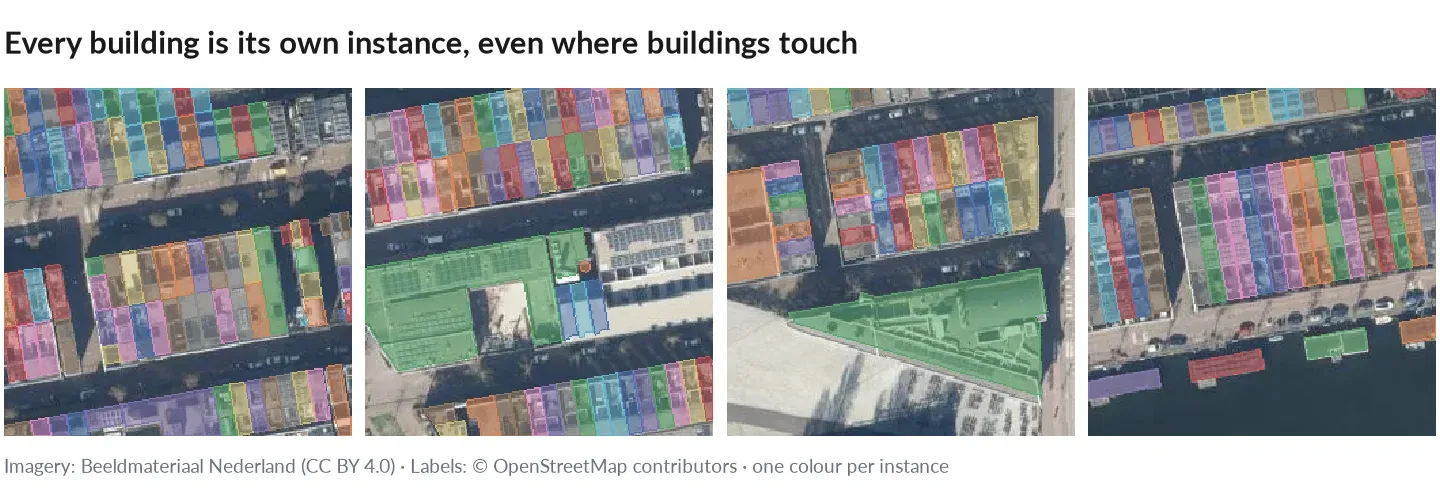
   Each building is its own instance, even where buildings touch. Shown with Dutch open aerial imagery (Beeldmateriaal Nederland, CC BY 4.0) over the same area; with the tutorial’s Esri imagery your patches look alike.

   Each COCO annotation has a segmentation in compressed RLE form, {"size": [256, 256], "counts": "…"}. pycocotools decodes it to the instance’s exact mask:

   look.py

   import matplotlib.pyplot as plt
   import numpy as np
   from PIL import Image
   from pycocotools.coco import COCO
   
   coco = COCO("dataset/annotations/instances_train.json")
   rng = np.random.default_rng(0)
   image_ids = [i for i in coco.getImgIds() if coco.getAnnIds(imgIds=[i])][:4]
   fig, axes = plt.subplots(1, len(image_ids), figsize=(4 * len(image_ids), 4))
   for ax, image_id in zip(axes, image_ids):
       info = coco.imgs[image_id]
       picture = np.asarray(Image.open(f"dataset/images/{info['file_name']}").convert("RGB")).copy()
       for ann in coco.loadAnns(coco.getAnnIds(imgIds=[image_id])):
           mask = coco.annToMask(ann).astype(bool)  # exactly this instance, even where it overlaps
           color = rng.integers(60, 255, size=3)
           picture[mask] = (0.5 * picture[mask] + 0.5 * color).astype(np.uint8)
       ax.imshow(picture)
       ax.set_title(info["file_name"])
       ax.axis("off")
   plt.tight_layout()
   plt.show()

   Every building gets its own colour. Footprints are drawn on other imagery, so tall buildings can look shifted (the photo shows them leaning).

   An annotation looks like this:

   {"id": 33, "image_id": 18, "category_id": 1, "segmentation": {"size": [256, 256], "counts": "baV13m78H00000^Vh0"}, "bbox": [154, 50, 5, 11], "area": 47, "iscrowd": 0, "truncated": false}

   bbox is the tight [x, y, width, height] of the mask in pixels, area its pixel count, and iscrowd is always 0. The file format is in Dataset format.

   The instance-ID PNGs. With id_mask: true, masks/patch_0000001.png is a 16-bit image the size of the patch: 0 is background and k marks the pixels of the k-th annotation of that image (annotations are numbered in the file’s order, which is the order of the label features). Where two instances overlap, the later one wins in this image, as later polygons overwrite earlier ones in a segmentation mask; the COCO masks are not affected. Read it with Pillow (np.array(Image.open(path)) gives uint16); a viewer that shows 16-bit images as black needs the values stretched.

   import numpy as np
   from PIL import Image
   
   ids = np.array(Image.open("dataset/masks/patch_0000001.png"))
   print(ids.dtype, ids.max())   # uint16 3: three buildings in this patch

   A patch with more than 65,535 instances cannot be stored in 16 bits: mapcv stops with an error that suggests a smaller patch_size, a larger min_area or id_mask: false.

6. Train a model

   torchvision Mask R-CNN reads the COCO files. This dataset class turns them into what the model expects (boxes as [x1, y1, x2, y2], one binary mask per instance, class IDs as labels, empty tensors for background patches):

   train_maskrcnn.py

   import json
   
   import numpy as np
   import torch
   import torchvision
   from PIL import Image
   from pycocotools import mask as mask_utils
   from torchvision.transforms.functional import to_tensor
   
   
   class CocoInstances(torch.utils.data.Dataset):
       def __init__(self, root, split):
           coco = json.load(open(f"{root}/annotations/instances_{split}.json"))
           self.root, self.images = root, coco["images"]
           self.anns = {image["id"]: [] for image in self.images}
           for ann in coco["annotations"]:
               self.anns[ann["image_id"]].append(ann)
   
       def __len__(self):
           return len(self.images)
   
       def __getitem__(self, index):
           image = self.images[index]
           anns = self.anns[image["id"]]
           height, width = image["height"], image["width"]
           masks = [mask_utils.decode(ann["segmentation"]) for ann in anns]  # (H, W) uint8
           boxes = [[x, y, x + w, y + h] for x, y, w, h in (ann["bbox"] for ann in anns)]
           target = {
               "boxes": torch.tensor(boxes, dtype=torch.float32).reshape(-1, 4),
               "labels": torch.tensor([ann["category_id"] for ann in anns], dtype=torch.int64),
               "masks": torch.from_numpy(
                   np.stack(masks) if masks else np.zeros((0, height, width), dtype=np.uint8)
               ),
           }
           pixels = Image.open(f"{self.root}/images/{image['file_name']}").convert("RGB")
           return to_tensor(pixels), target
   
   
   train = CocoInstances("dataset", "train")
   loader = torch.utils.data.DataLoader(
       train, batch_size=4, shuffle=True, collate_fn=lambda batch: tuple(zip(*batch))
   )
   # num_classes counts the background: 1 building class + 1.
   model = torchvision.models.detection.maskrcnn_resnet50_fpn(
       weights=None, weights_backbone="DEFAULT", num_classes=2
   )
   # torchvision's recipe scales the learning rate with the batch (0.02 for 16 images) and
   # warms it up; without the warmup the new mask head can diverge to NaN in the first epoch.
   optimizer = torch.optim.SGD(model.parameters(), lr=0.005, momentum=0.9, weight_decay=1e-4)
   warmup = torch.optim.lr_scheduler.LinearLR(optimizer, start_factor=0.01, total_iters=100)
   model.train()
   for epoch in range(20):
       for images, targets in loader:
           losses = model(list(images), list(targets))
           loss = sum(losses.values())
           optimizer.zero_grad()
           loss.backward()
           optimizer.step()
           warmup.step()
       print(epoch, loss.item())

   Detectron2 registers the files as they are:

   from detectron2.data.datasets import register_coco_instances
   
   for split in ("train", "val", "test"):
       register_coco_instances(
           f"buildings_{split}", {}, f"dataset/annotations/instances_{split}.json", "dataset/images"
       )

   For COCO-style mask AP on the test split, run the model on instances_test.json’s images and score the predictions with pycocotools.cocoeval.COCOeval(..., iouType="segm"); the area of each annotation is its mask’s pixel count, which COCO uses for its small/medium/large breakdown.

7. Variations

   • Several classes. Set label_field: building (the OSM tag: house, apartments, …) and a new staging_dir. COCO category_id is the class ID that mapcv plan prints.
   • Thin objects. labels.all_touched: true burns every pixel a footprint touches, which keeps narrow features (a 1 m wall at 0.4 m/px) from vanishing between pixel centres.
   • Large objects. A field or lake larger than a patch can never show 30% of itself in one patch; mapcv warns about such features. Lower min_visible, or use larger patches.
   • Boxes too. bbox is in every annotation, so the same dataset also trains a detector. For YOLO label files use task: detection instead.

Caution

A dataset’s instance settings are part of it: resuming with a different min_visible, min_area or id_mask (or a different labels.all_touched) is refused. Write to a new staging_dir instead. mapcv split re-splits a finished dataset and rewrites the COCO files, keeping every image and annotation ID.

Attribution

If you publish this dataset or a model trained on it, credit the sources: imagery by Esri World Imagery and labels © OpenStreetMap contributors (ODbL). See Providers & licensing.

Next

Dataset format → instance segmentation datasetsEvery field of the COCO RLE annotations, the ID masks and the manifest.