
Buildings from aerial imagery
This tutorial builds a building-segmentation dataset over Amsterdam’s Eastern Docklands at about 0.36 m per pixel, using Esri World Imagery tiles and building outlines from OpenStreetMap. Along the way you will learn how a config is put together, what plan and generate tell you, and how to switch from one class to many.
Time: about 15 minutes. You need: pip install mapcv, plus matplotlib for the optional visual check.
The finished files live in the repository under examples/quickstart. This page is self-contained, so you can also follow it from scratch.
-
Get the labels
Section titled “Get the labels”Labels are polygons in longitude/latitude. This tutorial uses OpenStreetMap buildings exported to GeoJSON (967 features, each with
class: buildingand the OSMbuildingtag):Terminal window mkdir docklands && cd docklandscurl -LO https://raw.githubusercontent.com/tahamukhtar20/mapcv/main/examples/quickstart/buildings.geojsonTo label your own area with OSM data, see Prepare labels → OpenStreetMap. OSM data is © OpenStreetMap contributors under the ODbL, which asks you to credit it when you share the result.
-
Write the config
Section titled “Write the config”Save this as
mapcv.yamlnext to the GeoJSON. Each block is explained below.mapcv.yaml region: # WGS-84 lon/lat; snapped outward to whole tileswest: 4.9375south: 52.3725east: 4.9515north: 52.3780imagery:type: xyzzoom: 18 # ≈ 0.36 m/px at this latitudesource: esri_satellitemax_connections: 4 # small and politelabels:path: buildings.geojsonlabel_field: class # every feature has class "building" -> mask value 1sampler:patch_size: 256 # one tile per patch at zoom 18edge_strategy: drop # the region is snapped to tiles, so nothing is droppedwriter:staging_dir: ./datasetimage_format: pngsplit:strategy: spatial # whole blocks go to one split: no leakage between splitstest_ratio: 0.20val_ratio: 0.10seed: 42regionis the area to cover, in degrees. mapcv expands it outward to whole 256 px tiles, so the raster is slightly larger than the box.imagerypicks the source.zoom: 18is roughly 0.36 m per pixel here; each zoom level halves the pixel size and quadruples the tile count. See Choose imagery and zoom.labels.label_fieldnames the GeoJSON property that holds the class. With a single value (building), it becomes class1; omit the field and every polygon is class1too, but the manifest then records no class names.samplercutspatch_sizesquares on a grid.stridedefaults to the patch size, so patches don’t overlap.splitwrites train/val/test lists.spatialassigns whole blocks of the map to one split, which is what you want for honest test scores (see Spatial leakage).
-
Validate and plan
Section titled “Validate and plan”mapcv validatechecks the YAML without touching the network or the label file;mapcv planalso reads the labels and estimates the job:Terminal window $ mapcv validate mapcv.yaml✓ mapcv.yaml is a valid config.Region 4.9375, 52.3725 → 4.9515, 52.378 (W, S → E, N)Imagery XYZ esri_satellite · zoom 18Labels buildings.geojson · field: classPatches 256 px · grid · stride 256 · edges: dropOutput dataset · pngSplit spatial · test 0.2 · val 0.1$ mapcv plan mapcv.yaml╭─ Plan for mapcv.yaml ────────────────────────────────────────────────────────────────╮│ Region 4.9375, 52.3725 → 4.9515, 52.378 (≈ 1.0 × 0.6 km) ││ Imagery esri_satellite · zoom 18 (≈ 0.36 m/px) ││ Raster 2,816 × 1,792 px · 77 tiles (≈ 1.9 MB to download) ││ Labels buildings.geojson · 967 polygons · classes: building → 1 ││ Patches ≈ 77 × 256 px (grid, stride 256) ││ Output dataset · png (≈ 8.6 MB) ││ Split spatial · test 0.2 · val 0.1 ││ Memory ≈ 28.8 MB per chunk │╰──────────────────────────────────────────────────────────────────────────────────────╯Read the plan before every real run.
classes: building → 1confirms the label field is right; a wrong field name shows up here as skipped features instead of as empty masks after a download. -
Generate
Section titled “Generate”Terminal window $ mapcv generate mapcv.yamlReading imagery and writing patches ━━━━━━━━━━━━━━━ 2/2 chunks • 0:00:06 • eta 0:00:00╭─ Dataset ready ──────────────────────────────────────────────────────────────────────╮│ Patches 77 ││ Source xyz · esri_satellite ││ Shape 256×256×3 uint8 ││ Tiles 77 fetched · 0 failed ││ Splits train 52 (68%) · val 8 (10%) · test 17 (22%) ││ Time 6s ││ Files dataset/ (Images/, Masks/, manifest.json, splits/, patches.geojson) │╰──────────────────────────────────────────────────────────────────────────────────────╯class id pixelsbackground 0 81.0%building 1 19.0%About 19 % of pixels are building: a typical class imbalance to keep in mind when you pick a loss.
Directorydataset/
DirectoryImages/ 77 × patch_0000000.png … (RGB)
- …
DirectoryMasks/ 77 × patch_0000000.png … (0 = background, 1 = building)
- …
- manifest.json
Directorysplits/
- train.txt 52 names
- val.txt 8 names
- test.txt 17 names
Directory10/ 20/ 30/ labeled/unlabeled subsets of train
- …
- patches.geojson footprints of the patches, to open in QGIS
-
Look at a few patches
Section titled “Look at a few patches”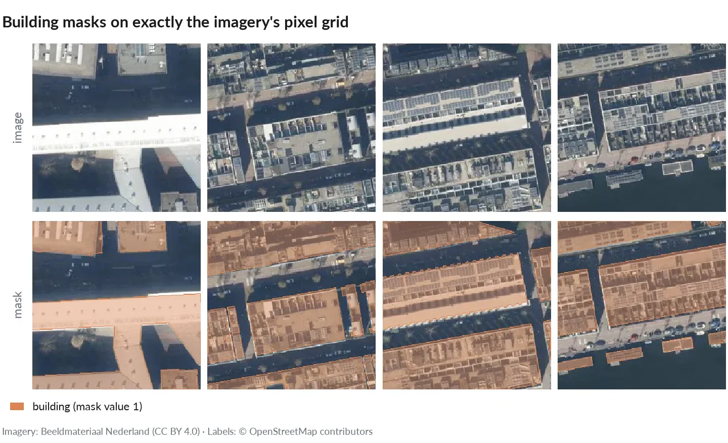
Four patches and their masks (yellow: building, mask value 1). Shown with Dutch open aerial imagery (Beeldmateriaal Nederland, CC BY 4.0) over the same area; with the tutorial’s Esri imagery your patches look alike.
Overlay masks on images to check alignment:
look.py import matplotlib.pyplot as pltimport numpy as npfrom PIL import Imagenames = open("dataset/splits/train.txt").read().split()[:4]fig, axes = plt.subplots(1, len(names), figsize=(4 * len(names), 4))for ax, name in zip(axes, names):image = np.asarray(Image.open(f"dataset/Images/{name}"))mask = np.asarray(Image.open(f"dataset/Masks/{name}"))ax.imshow(image)ax.imshow(np.ma.masked_equal(mask, 0), alpha=0.45, cmap="autumn")ax.set_title(name)ax.axis("off")plt.tight_layout()plt.show()Outlines should sit on roofs. OSM footprints are drawn on many different imagery sources, so expect small offsets on tall buildings (the aerial photo shows them leaning).
-
Try more classes
Section titled “Try more classes”The GeoJSON also carries the OSM
buildingtag (house,apartments,houseboat, …). Pointlabel_fieldat it and write to a new folder, because a dataset’s class map can’t change on resume:labels:path: buildings.geojsonlabel_field: buildingwriter:staging_dir: ./dataset-typesmapcv planshows the IDs it will use. Text labels are numbered in sorted order:Labels buildings.geojson · 967 polygons · classes: apartments → 1, church → 2,commercial → 3, garage → 4, house → 5, houseboat → 6, hut → 7, industrial →8, residential → 9, retail → 10, school → 11, service → 12, shed → 13, wall→ 14, yes → 15To group or pin classes, add
labels.classes; labels not listed are skipped (with a warning):labels:path: buildings.geojsonlabel_field: buildingclasses: {house: 1, apartments: 2, houseboat: 3}If you forget the new
staging_dir,generatestops before downloading anything:Cannot resume: dataset/manifest.json was generated with a different configuration(class_map, labels); use a new writer.staging_dir or remove the old dataset
Attribution
Section titled “Attribution”If you publish this dataset or a model trained on it, credit the sources: imagery by Esri World Imagery and labels © OpenStreetMap contributors (ODbL). See Providers & licensing.