Object detection datasets

This tutorial builds an object detection dataset from the quickstart data: Esri World Imagery over Amsterdam’s Eastern Docklands at about 0.36 m per pixel, with every OpenStreetMap building as a box. mapcv writes the boxes twice, as COCO JSON and as YOLO text files, so the same folder trains with Ultralytics, torchvision, Detectron2 or MMDetection.

Time: about 15 minutes. You need: pip install mapcv; ultralytics or torch + torchvision for the training step.

1. Get the labels

   The labels are the quickstart’s building outlines (967 features, each with class: building):

   mkdir docklands-boxes && cd docklands-boxes
   curl -LO https://raw.githubusercontent.com/tahamukhtar20/mapcv/main/examples/quickstart/buildings.geojson

   OSM data is © OpenStreetMap contributors under the ODbL, which asks you to credit it when you share the result.

2. Write the config

   It is the quickstart config plus task: detection and an optional detection block. mapcv init --template detection writes the same file with comments.

   mapcv.yaml

   task: detection
   
   region:
     west: 4.9375
     south: 52.3725
     east: 4.9515
     north: 52.3780
   
   imagery:
     type: xyz
     zoom: 18                   # ≈ 0.36 m/px at this latitude
     source: esri_satellite
     max_connections: 4
   
   labels:
     path: buildings.geojson
     label_field: class         # one class: building
   
   detection:
     min_visible: 0.3           # keep a building in a patch if ≥ 30% of it is visible there
     min_box_pixels: 2          # drop slivers narrower or shorter than 2 px
     formats: [coco, yolo]
   
   sampler:
     patch_size: 256
     edge_strategy: drop
   
   writer:
     staging_dir: ./dataset
     image_format: png
   
   split:
     strategy: spatial          # whole blocks per split: no leakage between splits
     test_ratio: 0.20
     val_ratio: 0.10
     seed: 42

   How a building becomes a box:

   • One feature, one object. Each GeoJSON feature is one object, including a MultiPolygon. A building cut by a patch edge is still one object; its box covers the part inside the patch.
   • Only what is visible. The box surrounds the part of the building that the patch shows: inside the patch, inside the raster, and over pixels that have imagery (failed tiles and NoData are cut out). Courtyards (holes) do not change the box.
   • min_visible decides whether a building that the patch shows only in part gets a box there. With 0.3, a building split 50/50 between two patches gets a box in both, and one with 20% in a patch gets none in that patch. Boxes of cut buildings are flagged truncated in COCO.
   • min_box_pixels removes thin slivers along patch edges.

   All options: Configuration → detection.

3. Plan

   $ mapcv plan mapcv.yaml
   ╭─ Plan for mapcv.yaml ────────────────────────────────────────────────────────╮
   │ Task     detection · coco, yolo · min_visible 0.3 · boxes ≥ 2 px             │
   │ Region   4.9375, 52.3725 → 4.9515, 52.378  (≈ 1.0 × 0.6 km)                  │
   │ Imagery  esri_satellite · zoom 18 (≈ 0.36 m/px)                              │
   │ Raster   2,816 × 1,792 px · 77 tiles (≈ 1.9 MB to download)                  │
   │ Labels   buildings.geojson · 967 polygons · classes: building → 1            │
   │ Patches  ≈ 77 × 256 px (grid, stride 256)                                    │
   │ Objects  ≈ 670 (label features in the region; one box each, in every patch   │
   │          that shows enough of it)                                            │
   │ Output   dataset · png (≈ 8.5 MB)                                            │
   │ Split    spatial · test 0.2 · val 0.1                                        │
   │ Memory   ≈ 28.8 MB per chunk                                                 │
   ╰──────────────────────────────────────────────────────────────────────────────╯

   670 of the 967 buildings lie in the region. Buildings that cross patch edges can get a box in two or more patches, so the dataset will hold more boxes than that.

4. Generate

   $ mapcv generate mapcv.yaml
   ╭─ Dataset ready ──────────────────────────────────────────────────────────────╮
   │ Patches  77                                                                  │
   │ Source   xyz · esri_satellite                                                │
   │ Shape    256×256×3 uint8                                                     │
   │ Tiles    77 fetched · 0 failed                                               │
   │ Splits   train 52 (68%) · val 8 (10%) · test 17 (22%)                        │
   │ Time     6s                                                                  │
   │ Files    dataset/ (images/, manifest.json, splits/, patches.geojson,         │
   │          annotations/, labels/, train.txt, val.txt, test.txt, dataset.yaml)  │
   ╰──────────────────────────────────────────────────────────────────────────────╯
     class       id    objects     share    patches
     building     1        800    100.0%         58

   800 boxes in 58 patches; the other 19 patches (water, quays) have no buildings and stay in the dataset as background images. mapcv info dataset shows the same table later.

   • Directorydataset/

     • Directoryimages/ 77 × patch_0000000.png …

       • …
     • Directorylabels/ YOLO: 58 × patch_0000000.txt … (none for patches without buildings)

       • …
     • Directoryannotations/

       • instances_train.json COCO: 52 images, 413 boxes
       • instances_val.json 8 images, 79 boxes
       • instances_test.json 17 images, 308 boxes
       • Directoryobjects/ mapcv’s own record of the boxes, used to resume and re-split

         • …
     • train.txt val.txt test.txt image lists for YOLO
     • dataset.yaml Ultralytics dataset file
     • manifest.json
     • Directorysplits/ the split as patch names, as for segmentation

       • …
     • patches.geojson footprints of the patches, to open in QGIS

5. Look at the boxes

   

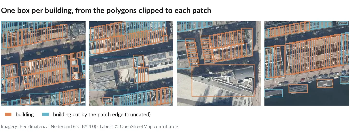
   Boxes from the COCO file: buildings cut by the patch edge (truncated) in blue. Shown with Dutch open aerial imagery (Beeldmateriaal Nederland, CC BY 4.0) over the same area; with the tutorial’s Esri imagery your patches look alike.

   COCO boxes are [x, y, width, height] in pixels from the patch’s top-left corner:

   look.py

   import json
   
   import matplotlib.patches as patches
   import matplotlib.pyplot as plt
   from PIL import Image
   
   coco = json.load(open("dataset/annotations/instances_train.json"))
   images = coco["images"][:4]
   fig, axes = plt.subplots(1, len(images), figsize=(4 * len(images), 4))
   for ax, image in zip(axes, images):
       ax.imshow(Image.open(f"dataset/images/{image['file_name']}"))
       for ann in coco["annotations"]:
           if ann["image_id"] == image["id"]:
               x, y, w, h = ann["bbox"]
               color = "orange" if ann["truncated"] else "lime"
               ax.add_patch(patches.Rectangle((x, y), w, h, fill=False, color=color))
       ax.set_title(image["file_name"])
       ax.axis("off")
   plt.tight_layout()
   plt.show()

   Boxes should frame roofs; orange ones are buildings cut by the patch edge. Footprints are drawn on other imagery, so tall buildings can look shifted (the photo shows them leaning).

6. Train a detector

   Ultralytics YOLO reads dataset.yaml, which points at the image lists and names the classes (0: building):

   pip install ultralytics
   yolo detect train data=dataset/dataset.yaml model=yolo11n.pt imgsz=256 epochs=50

   or from Python:

   from ultralytics import YOLO
   
   model = YOLO("yolo11n.pt")
   model.train(data="dataset/dataset.yaml", imgsz=256, epochs=50)
   metrics = model.val(split="test")

   dataset.yaml has no path: key, so Ultralytics resolves the image lists against the folder the file is in: copy the whole dataset/ folder to a GPU machine and train there without editing anything.

   torchvision reads the COCO files. This dataset class turns them into what torchvision’s detection models expect (boxes as [x1, y1, x2, y2], class IDs as labels, and an empty box list for background patches):

   train_frcnn.py

   import json
   
   import torch
   import torchvision
   from PIL import Image
   from torchvision.transforms.functional import to_tensor
   
   
   class CocoBoxes(torch.utils.data.Dataset):
       def __init__(self, root, split):
           coco = json.load(open(f"{root}/annotations/instances_{split}.json"))
           self.root, self.images = root, coco["images"]
           self.boxes = {image["id"]: [] for image in self.images}
           for ann in coco["annotations"]:
               self.boxes[ann["image_id"]].append(ann)
   
       def __len__(self):
           return len(self.images)
   
       def __getitem__(self, index):
           image = self.images[index]
           anns = self.boxes[image["id"]]
           boxes = [[x, y, x + w, y + h] for x, y, w, h in (ann["bbox"] for ann in anns)]
           target = {
               "boxes": torch.tensor(boxes, dtype=torch.float32).reshape(-1, 4),
               "labels": torch.tensor([ann["category_id"] for ann in anns], dtype=torch.int64),
           }
           pixels = Image.open(f"{self.root}/images/{image['file_name']}").convert("RGB")
           return to_tensor(pixels), target
   
   
   train = CocoBoxes("dataset", "train")
   loader = torch.utils.data.DataLoader(
       train, batch_size=8, shuffle=True, collate_fn=lambda batch: tuple(zip(*batch))
   )
   # num_classes counts the background: 1 building class + 1.
   model = torchvision.models.detection.fasterrcnn_resnet50_fpn(
       weights=None, weights_backbone="DEFAULT", num_classes=2
   )
   optimizer = torch.optim.SGD(model.parameters(), lr=0.01, momentum=0.9, weight_decay=1e-4)
   model.train()
   for epoch in range(20):
       for images, targets in loader:
           losses = model(list(images), list(targets))
           loss = sum(losses.values())
           optimizer.zero_grad()
           loss.backward()
           optimizer.step()
       print(epoch, loss.item())

   For COCO-style mAP on the test split, run the model on instances_test.json’s images and score the results with pycocotools.cocoeval.COCOeval; the area of each annotation is the building’s visible area, which COCO uses for its small/medium/large breakdown.

7. Variations

   • Several classes. Set label_field: building (the OSM tag: house, apartments, …) and a new staging_dir. COCO category_id is the class ID that mapcv plan prints; YOLO indices are the same classes counted from 0 in ID order.
   • Points. For point labels (trees, cars, wells), set detection.point_box_size to a box side in pixels: each point (GeoJSON, GeoPackage, Shapefile or GeoParquet) becomes a square box centred on it.
   • Only one format. formats: [yolo] or formats: [coco].
   • Large objects. A field or lake larger than a patch can never show 30% of itself in one patch; mapcv warns about such features. Lower min_visible, or use larger patches.

Caution

A dataset’s detection settings are part of it: resuming with a different min_visible, min_box_pixels, formats or point_box_size is refused. Write to a new staging_dir instead. mapcv split re-splits a finished dataset and rewrites the COCO files, image lists and dataset.yaml, keeping every image and annotation ID.

Attribution

If you publish this dataset or a model trained on it, credit the sources: imagery by Esri World Imagery and labels © OpenStreetMap contributors (ODbL). See Providers & licensing.

Next

Dataset format → detection datasetsEvery field of the COCO, YOLO and manifest files.