Land cover from Sentinel-2

This tutorial builds a multispectral land-cover dataset near Amerongen in the Netherlands: red, green, blue and near-infrared Sentinel-2 bands at 10 m, labeled with four classes (built-up, farmland, forest, water) from OpenStreetMap, cut into 128 × 128 patches stored as float32 NumPy arrays.

Time: about 15 minutes, most of it waiting for the product to stream. You need: Python 3.10–3.13 and an internet connection.

The finished files are in examples/sentinel2-landcover; this page is self-contained.

Install the Sentinel-2 extra
Section titled “Install the Sentinel-2 extra”
Terminal window
```
pip install "mapcv[zarr]"
```
This adds xarray-eopf, xarray, Dask, zarr 2, numba, pyproj, s3fs and pystac-client. On Python 3.14 the extra installs nothing (see Installation).
Pick a product
Section titled “Pick a product”

An eopf_zarr source reads one Sentinel-2 L2A product in ESA’s EOPF Zarr format (imagery.search can also find the least cloudy one for you). Find one in the EOPF STAC browser (collection sentinel-2-l2a): filter by your area and date, sort by cloud cover, and copy the product’s .zarr link. This tutorial uses an almost cloud-free scene from 13 May 2025 (tile 31UFT, 0.03 % cloud):
```
https://objectstore.eodc.eu:2222/e05ab01a9d56408d82ac32d69a5aae2a:202505-s02msil2a/13/products/cpm_v256/S2A_MSIL2A_20250513T104041_N0511_R008_T31UFT_20250513T143716.zarr
```
No account or key is needed. Copernicus Sentinel data is free and open; credit it as “Contains modified Copernicus Sentinel data [2025]”.
Get the labels
Section titled “Get the labels”
Terminal window
```
mkdir s2-landcover && cd s2-landcover
curl -LO https://raw.githubusercontent.com/tahamukhtar20/mapcv/main/examples/sentinel2-landcover/landuse.geojson
```
The file holds 643 OpenStreetMap land-use, forest and water polygons (© OpenStreetMap contributors, ODbL), already grouped into a class property with four values. To make your own, see Prepare labels.

Write the config

Start from mapcv init mapcv.yaml --template sentinel2, or save this directly:

region:                      # WGS-84 lon/lat, inside the product's footprint
  west: 5.400
  south: 51.975
  east: 5.500
  north: 52.035

imagery:
  type: eopf_zarr
  path: https://objectstore.eodc.eu:2222/e05ab01a9d56408d82ac32d69a5aae2a:202505-s02msil2a/13/products/cpm_v256/S2A_MSIL2A_20250513T104041_N0511_R008_T31UFT_20250513T143716.zarr
  resolution: 10             # metres; the 10 m bands are b02, b03, b04 and b08
  bands: [b04, b03, b02, b08]   # red, green, blue, near-infrared, in this order

labels:
  path: landuse.geojson
  label_field: class
  classes:                   # pin the mask values instead of relying on sorted order
    built_up: 1
    farmland: 2
    forest: 3
    water: 4

sampler:
  patch_size: 128            # 1.28 km per patch at 10 m
  edge_strategy: drop
  max_empty_ratio: 0.2       # skip patches with more than 20 % NoData (NaN)

writer:
  staging_dir: ./dataset
  image_format: npy          # float32, bands-first: (4, 128, 128)

split:
  strategy: spatial
  test_ratio: 0.20
  val_ratio: 0.10
  seed: 42

What differs from an XYZ config:

imagery.bands sets both which bands are read and their order in every array. Omit it for all 12 L2A bands.
resolution is the output grid; bands with a coarser native resolution are resampled onto it.
image_format: npy (or tif, for georeferenced GeoTIFF patches) is required: reflectance is float32 with NaN for no data, which PNG can’t store.
edge_strategy: drop and max_empty_ratio: 0.2 avoid zero-padded and mostly-NaN patches at the edges.

Plan

$ mapcv plan mapcv.yaml
╭─ Plan for mapcv.yaml ────────────────────────────────────────────────────────────────╮
│ Region   5.4, 51.975 → 5.5, 52.035  (≈ 6.9 × 6.6 km)                                 │
│ Imagery  Sentinel-2 L2A (EOPF) · 4 bands (≈ 10.00 m/px)                              │
│ Raster   709 × 692 px                                                                │
│ Labels   landuse.geojson · 643 polygons · classes: built_up → 1, farmland → 2,       │
│          forest → 3, water → 4                                                       │
│ Patches  ≈ 25 × 128 px (grid, stride 128)                                            │
│ Output   dataset · npy (≈ 6.6 MB)                                                    │
│ Split    spatial · test 0.2 · val 0.1                                                │
│ Memory   ≈ 16.7 MB per chunk                                                         │
╰──────────────────────────────────────────────────────────────────────────────────────╯

For Sentinel-2 the raster size is computed on the region’s UTM grid; the product’s exact grid is known once it is opened.

Generate

$ mapcv generate mapcv.yaml
  Reading imagery and writing patches ━━━━━━━━━━━━━━━ 1/1 chunks • 0:01:11 • eta 0:00:00
╭─ Dataset ready ──────────────────────────────────────────────────────────────────────╮
│ Patches  25                                                                          │
│ Source   eopf_zarr ·                                                                 │
│          S2A_MSIL2A_20250513T104041_N0511_R008_T31UFT_20250513T143716.zarr           │
│ Shape    4×128×128 float32                                                           │
│ Splits   train 18 (72%) · val 2 (8%) · test 5 (20%)                                  │
│ Time     1m 47s                                                                      │
│ Files    dataset/ (Images/, Masks/, manifest.json, splits/, patches.geojson)         │
╰──────────────────────────────────────────────────────────────────────────────────────╯
  class         id    pixels
  background     0     25.7%
  built_up       1      7.8%
  farmland       2     19.0%
  forest         3     42.9%
  water          4      4.7%

About a quarter of the pixels are background: land that none of the four classes covers.

Inspect

$ mapcv info dataset
╭─ dataset ────────────────────────────────────────────────────────────────────────────╮
│ Task      segmentation                                                               │
│ Source    eopf_zarr ·                                                                │
│           S2A_MSIL2A_20250513T104041_N0511_R008_T31UFT_20250513T143716.zarr          │
│ Bands     b04, b03, b02, b08                                                         │
│ Patches   25 · 4×128×128 float32                                                     │
│ CRS       EPSG:32631                                                                 │
│ Ignore    mask value 255 marks pixels without imagery                                │
│ Splits    train 18 (72%) · val 2 (8%) · test 5 (20%)                                 │
│ Manifest  version 3                                                                  │
╰──────────────────────────────────────────────────────────────────────────────────────╯

The patches are in the product’s own UTM zone (EPSG:32631), not Web Mercator: mapcv reprojected the labels into it rather than resampling the imagery. See Coordinates and grids.

Look at the bands

Three Sentinel-2 true-colour patches near Utrecht, and the same patches with built-up, farmland, forest and water masks

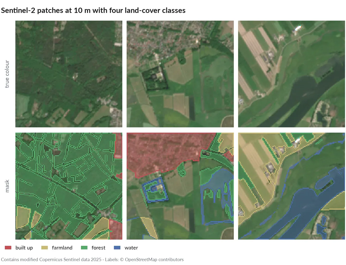
Patches from this tutorial’s product as true colour (b04, b03, b02, stretched) and with their masks. Contains modified Copernicus Sentinel data 2025; labels © OpenStreetMap contributors.

import json
import numpy as np
from PIL import Image

manifest = json.load(open("dataset/manifest.json"))
bands = manifest["sources"][0]["bands"]            # ['b04', 'b03', 'b02', 'b08']
class_map = manifest["target"]["class_map"]
names = {cid: name for name, cid in class_map.items()} | {0: "background", 255: "no data"}

files = manifest["patches"][0]["files"]            # paths relative to dataset/
image = np.load(f"dataset/{files['image']}")       # (4, 128, 128) float32 reflectance
mask = np.asarray(Image.open(f"dataset/{files['mask']}"))

red, nir = image[bands.index("b04")], image[bands.index("b08")]
ndvi = (nir - red) / (nir + red + 1e-6)
for cid in np.unique(mask):
    print(f"{names[int(cid)]:<10} mean NDVI {np.nanmean(ndvi[mask == cid]):.2f}")

rgb = np.clip(np.moveaxis(image[[0, 1, 2]], 0, -1) * 3.5, 0, 1)   # simple true-colour stretch

On the first patch it prints (order follows the class IDs):

background mean NDVI 0.75
built_up   mean NDVI 0.68
farmland   mean NDVI 0.65
forest     mean NDVI 0.83

Forest is the greenest. Farmland can be as low as built-up land in summer, when fields are harvested or bare. Treat NaN as no data in anything you compute.

Things to try

More bands: remove bands to get all 12 at 10 m, or set resolution: 20 for the red-edge and SWIR bands at their native grid. Use a new staging_dir: band changes can’t be resumed into the old folder.
Bigger patches or overlap: patch_size: 256, or stride: 64 with the default spatial split, which leaves out train/val patches overlapping test.
Another date: swap imagery.path for a product from a different season and compare class separability.

Attribution

Credit “Contains modified Copernicus Sentinel data [2025]” for the imagery and “© OpenStreetMap contributors” (ODbL) for the labels. See Providers & licensing.

Train a model on your datasetFeed these patches into a PyTorch training loop.

Land cover from Sentinel-2

Install the Sentinel-2 extra

Pick a product

Get the labels