Patch classification datasets

This tutorial builds a scene classification dataset in the style of EuroSAT and BigEarthNet: Esri World Imagery near Amerongen in the Netherlands at about 1.5 m per pixel, cut into 128 × 128 patches (about 190 m wide), each labeled with the land use that covers most of it: built-up, farmland, forest or water. mapcv decides the label from the share of every patch that each OpenStreetMap polygon class covers, and writes the labels as a CSV and a JSON file next to the images.

Time: about 10 minutes. You need: pip install mapcv; torch + torchvision for the training step.

1. Get the labels

   The labels are the 643 land-use, forest and water polygons of the Sentinel-2 example, grouped into a class property with four values:

   mkdir landuse-scenes && cd landuse-scenes
   curl -LO https://raw.githubusercontent.com/tahamukhtar20/mapcv/main/examples/sentinel2-landcover/landuse.geojson

   OSM data is © OpenStreetMap contributors under the ODbL, which asks you to credit it when you share the result.

2. Write the config

   It is a segmentation config plus task: classification and an optional classification block. mapcv init --template classification writes a commented starting point.

   mapcv.yaml

   task: classification
   
   region:
     west: 5.400
     south: 51.975
     east: 5.500
     north: 52.035
   
   imagery:
     type: xyz
     zoom: 16                   # ≈ 1.5 m/px at this latitude
     source: esri_satellite
     max_connections: 4
   
   labels:
     path: landuse.geojson
     label_field: class         # built_up, farmland, forest, water
   
   classification:
     mode: single               # one label per patch
     min_fraction: 0.5          # the class must cover at least half of the patch
     empty: skip                # drop patches no class covers that much
   
   sampler:
     patch_size: 128            # ≈ 190 m per patch
     edge_strategy: drop
   
   writer:
     staging_dir: ./dataset
     image_format: png
   
   split:
     strategy: spatial          # whole blocks per split: no leakage between splits
     test_ratio: 0.20
     val_ratio: 0.10
     seed: 42

   How a patch gets its label:

   • Coverage. mapcv burns the labels into the same class mask that task: segmentation would write, with the same rasterizer and pixel rule, and counts the pixels of each class. A class’s coverage is its pixels divided by the patch’s valid pixels: pixels that have imagery (not NoData, not a failed tile, not padding) and are not labels.ignore_index. Where polygons overlap, the later one in the file wins, as in a segmentation mask.
   • single gives the patch the class with the largest coverage (a tie goes to the lowest class ID), as long as that class reaches min_fraction. multi gives it every class that reaches min_fraction.
   • min_fraction is inclusive, and 0 means “any labeled pixel”: a class qualifies when its coverage is at least this and above zero.
   • empty says what happens to a patch no class qualifies for: skip drops it, background keeps it with the label background.

   All options: Configuration → classification.

3. Plan

   $ mapcv plan mapcv.yaml
   ╭─ Plan for mapcv.yaml ────────────────────────────────────────────────────────╮
   │ Task     classification · single-label · min_fraction 0.5 · empty: skip      │
   │ Region   5.4, 51.975 → 5.5, 52.035  (≈ 6.9 × 6.6 km)                         │
   │ Imagery  esri_satellite · zoom 16 (≈ 1.47 m/px)                              │
   │ Raster   4,864 × 4,608 px · 342 tiles (≈ 8.6 MB to download)                 │
   │ Labels   landuse.geojson · 643 polygons · classes: built_up → 1, farmland →  │
   │          2, forest → 3, water → 4                                            │
   │ Patches  ≈ 1,368 × 128 px (grid, stride 128)                                 │
   │ Output   dataset · png (≈ 37.3 MB)                                           │
   │ Split    spatial · test 0.2 · val 0.1                                        │
   │ Memory   ≈ 44.8 MB per chunk                                                 │
   ╰──────────────────────────────────────────────────────────────────────────────╯

   The plan counts every grid position. Patches that no class covers by at least half are dropped when the dataset is built, so it will hold fewer.

4. Generate

   $ mapcv generate mapcv.yaml
   ╭─ Dataset ready ──────────────────────────────────────────────────────────────╮
   │ Patches  984                                                                 │
   │ Source   xyz · esri_satellite                                                │
   │ Shape    128×128×3 uint8                                                     │
   │ Tiles    342 fetched · 0 failed                                              │
   │ Splits   train 700 (71%) · val 81 (8%) · test 203 (21%)                      │
   │ Time     51s                                                                 │
   │ Files    dataset/ (images/, manifest.json, splits/, patches.geojson,         │
   │          labels.csv, labels_train.csv, labels_val.csv, labels_test.csv,      │
   │          labels.json, classes.txt)                                           │
   ╰──────────────────────────────────────────────────────────────────────────────╯
     label       id    patches    share
     built_up     1        106    10.8%
     farmland     2        228    23.2%
     forest       3        590    60.0%
     water        4         60     6.1%

   984 of the 1,368 grid positions had a class over half of them; the rest are mixed or unlabeled and were skipped. mapcv info dataset shows the same table later.

   • Directorydataset/

     • Directoryimages/ 984 × patch_0000000.png …

       • …
     • labels.csv image,labels,split for every patch
     • labels_train.csv image,labels of the 700 train patches
     • labels_val.csv 81 val patches
     • labels_test.csv 203 test patches
     • classes.txt built_up, farmland, forest, water: one per line
     • labels.json the classes and every image’s labels
     • manifest.json
     • Directorysplits/ the split as patch names, as for every task

       • …
     • patches.geojson footprints of the patches, to open in QGIS

   labels.csv is one row per patch:

   dataset/labels.csv

   image,labels,split
   patch_0000000.png,forest,train
   patch_0000001.png,forest,train
   patch_0000002.png,forest,train

   labels.json holds the same labels as arrays, so a multi-label dataset needs no parsing:

   dataset/labels.json

   {
     "classes": ["built_up", "farmland", "forest", "water"],
     "images": {
       "patch_0000000.png": ["forest"],
       "patch_0000001.png": ["forest"],
       …

   manifest.json records every patch’s coverage per class and its labels, so you can pick a stricter threshold later without touching the imagery:

   {"row":0,"col":0,"padded":false,"chunk":0,"files":{"image":"images/patch_0000000.png"},"summary":{"class_coverage":{"3":0.912109375},"labels":[3],"empty_ratio":0.0}}

5. Look at the patches

   

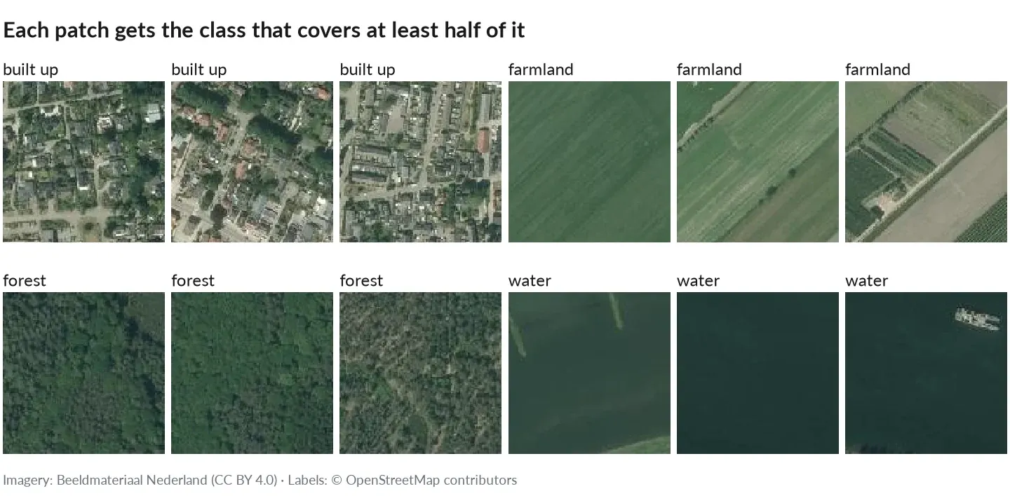
   Three patches per class, each covered by its class for at least half its area. Shown with Dutch open aerial imagery (Beeldmateriaal Nederland, CC BY 4.0) over the same area; with the tutorial’s Esri imagery your patches look alike.

   look.py

   import csv
   import random
   
   import matplotlib.pyplot as plt
   from PIL import Image
   
   with open("dataset/labels_train.csv", newline="", encoding="utf-8") as handle:
       rows = list(csv.DictReader(handle))
   
   random.seed(0)
   by_label = {}
   for row in rows:
       by_label.setdefault(row["labels"], []).append(row["image"])
   
   fig, axes = plt.subplots(len(by_label), 4, figsize=(8, 2 * len(by_label)))
   for line, (label, images) in zip(axes, sorted(by_label.items())):
       for ax, image in zip(line, random.sample(images, 4)):
           ax.imshow(Image.open(f"dataset/images/{image}"))
           ax.axis("off")
       line[0].set_title(f"{label} ({len(images)})", loc="left", fontsize=9)
   plt.tight_layout()
   plt.show()

   The rows are the four classes (59, 132, 462 and 47 train patches). A label is only as good as the polygons: OSM’s forest polygons contain clearings and a few houses, and a farmland patch can hold a corner of a pond. That is why min_fraction: 0.5 is a sensible start; raise it for cleaner, rarer examples.

6. Train a classifier

   labels_train.csv and labels_val.csv are everything a loader needs. This dataset class reads a split and returns an image with its class index (the position of the name in classes.txt):

   train_classifier.py

   import csv
   
   import torch
   import torchvision
   from PIL import Image
   from torchvision.transforms.functional import to_tensor
   
   ROOT = "dataset"
   classes = open(f"{ROOT}/classes.txt", encoding="utf-8").read().splitlines()
   index = {name: i for i, name in enumerate(classes)}
   
   
   class Scenes(torch.utils.data.Dataset):
       def __init__(self, split):
           with open(f"{ROOT}/labels_{split}.csv", newline="", encoding="utf-8") as handle:
               self.rows = list(csv.DictReader(handle))
   
       def __len__(self):
           return len(self.rows)
   
       def __getitem__(self, i):
           row = self.rows[i]
           image = Image.open(f"{ROOT}/images/{row['image']}").convert("RGB")
           return to_tensor(image), index[row["labels"]]
   
   
   train = torch.utils.data.DataLoader(Scenes("train"), batch_size=32, shuffle=True)
   val = torch.utils.data.DataLoader(Scenes("val"), batch_size=64)
   
   model = torchvision.models.resnet18(weights="DEFAULT")
   model.fc = torch.nn.Linear(model.fc.in_features, len(classes))
   optimizer = torch.optim.AdamW(model.parameters(), lr=1e-3)
   loss_fn = torch.nn.CrossEntropyLoss()
   
   for epoch in range(10):
       model.train()
       for images, labels in train:
           loss = loss_fn(model(images), labels)
           optimizer.zero_grad()
           loss.backward()
           optimizer.step()
       model.eval()
       correct = 0
       with torch.no_grad():
           for images, labels in val:
               correct += (model(images).argmax(1) == labels).sum().item()
       print(epoch, loss.item(), correct / len(val.dataset))

   The classes are unbalanced (60 % forest), so look at per-class recall, not only accuracy, and consider a weighted loss. Evaluate once on labels_test.csv at the end.

7. Variations

   • Several labels per patch. Set mode: multi, min_fraction: 0.1 and empty: background: a patch gets every class that covers at least 10 % of it, and a patch with no such class is kept as background. On the same area that makes 1,368 patches, among them 149 background, 598 forest only, 105 farmland forest and a few with three classes. labels.csv then holds the names joined by a space, and classes.txt starts with background:

     dataset/labels.csv

     image,labels,split
     patch_0000000.png,forest,train
     patch_0000007.png,farmland forest,test
     patch_0000010.png,background,train
     patch_0000423.png,built_up farmland,train

     Turn labels.json into multi-hot targets with classes for the column order, and train with BCEWithLogitsLoss:

     import json
     
     import torch
     
     data = json.load(open("dataset/labels.json"))
     index = {name: i for i, name in enumerate(data["classes"])}
     
     
     def multi_hot(names):
         target = torch.zeros(len(index))
         for name in names:
             target[index[name]] = 1.0
         return target

     In multi mode class names cannot contain whitespace (it separates the labels in the CSV); mapcv stops with a message that names the class if one does.

   • Any pixel counts. With the default min_fraction: 0, a patch gets a label as soon as one valid pixel is labeled. Useful for rare classes such as a road or a pond that cover little of a patch; combine it with multi.

   • Label rasters. labels.type: raster works too: the label raster is sampled onto each patch exactly as for segmentation, and the classes you declare in labels.classes become the labels (use name: to choose them). Pixels outside the label raster, on its NoData or on ignore_values are not valid and do not count.

   • Re-split without regenerating. mapcv split dataset --strategy spatial --test-ratio 0.3 rewrites the split column of labels.csv and the three labels_<split>.csv files from the manifest. With --strategy stratified the strata come from each patch’s label (for several labels, the one with the largest coverage), so every class is spread over the splits in proportion.

Caution

A dataset’s classification settings are part of it: resuming with a different mode, min_fraction or empty (or labels.all_touched) is refused. Write to a new staging_dir instead. Patches without a single valid pixel (all NoData or failed tiles) are never labeled; use sampler.max_empty_ratio to also drop patches that are mostly without imagery, since a label over a few valid pixels is a poor one.

Attribution

If you publish this dataset or a model trained on it, credit the sources: imagery by Esri World Imagery and labels © OpenStreetMap contributors (ODbL). See Providers & licensing.

Next

Dataset format → classification datasetsEvery column of the CSV, JSON and manifest files.